Graphing Time
The biggest challenge I encountered when translating timetables into graph data involved temporal elements - that is, start and end times, dates, weeks, recurrences, durations, etc. While the basic model successfully captured the core entities and relationships, it lacked the necessary detail to perform meaningful time-based analysis.
The flexibility of graph databases is appealing but finding the optimal balance between efficient representation, query performance, and data redundancy requires careful consideration. This section details some challenges encountered and the approach taken for the proof-of-concept.
The Problem of Normalised Time
Traditional relational databases often store timetable information in a highly normalised1 format, condensing recurring events into single rows with date ranges, week patterns, or lists of occurrences. While efficient for storage and basic display, this approach severely hinders analysis, especially when aiming to:
- Identify Time-Based Patterns: Determining if students lack lunch breaks or experience excessive gaps between classes becomes difficult when time is fragmented across multiple fields.
- Perform Aggregations: Calculating total teaching hours for a lecturer across specific weeks or days requires complex queries and data transformations.
- Model Temporal Relationships: Representing relationships between activities based on their temporal proximity, such as students attending consecutive classes, becomes convoluted.
Exploring Potential Solutions
Several time modelling approaches were considered, each with its own trade-offs.
To illustrate this, let’s explore using a fictional example - Introduction to Graph Databases - focusing on the lecture:
| Name | Activity Type | Day | StartTime | EndTime | Weeks |
|---|---|---|---|---|---|
| ITGD | Lecture | Wednesday | 09:00 | 11:00 | 1-3, 5-7, 9-13 |
| ITGD | Seminar | Wednesday | 10:00 | 13:00 | 4, 7-8, 15 |
| ITGD | Seminar | Monday | 13:00 | 16:00 | 4, 7-8, 15 |
Option 0: Proof-of-concept activity
The basic model creates nodes for each activity exactly as they exist in the relational database. This simple approach is perfectly acceptable but makes any time-based calculations difficult because each activity node can represent a different number of occurrences due to the week ranges.
This in turn means you cannot simply COUNT each activity “equally” - for example, the lecture has 11 instances, each of two hours. The seminars have four instances, each of three hours. Calculating aggregations, finding clashes and similar is very challenging.
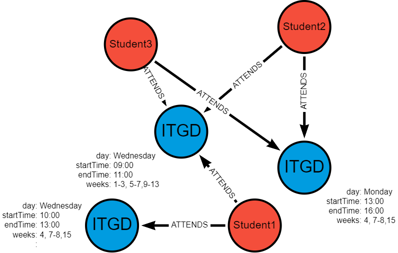
If we assume that each student attends the lecture and one of the seminars, some students have a clash in week 7 (Wednesday 10:00-11:00) - this is very difficult to identify and isolate in a highly normalised dataset.
Option 1: Unique Activity Nodes
Option 1 addresses this by creating nodes for each unique combination of name, startTime, endTime and date - this means de-normalising the relational data and deliberately introducing duplication.
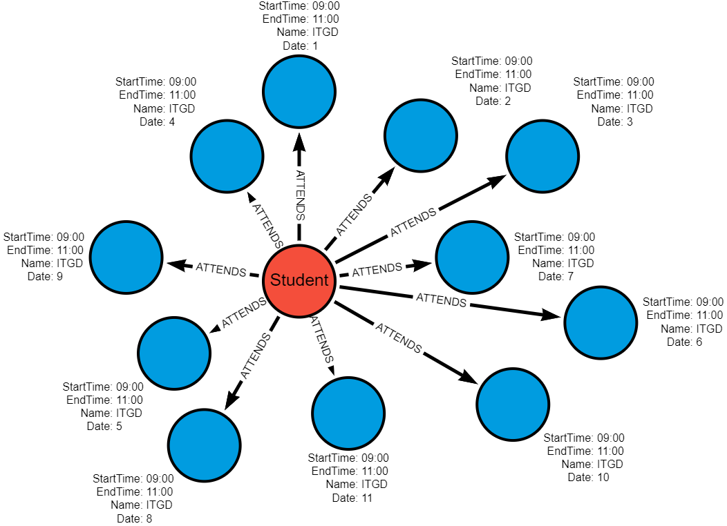
Graph Structure:
- 11 separate
Activitynodes one for each occurrence (date) - Each node has
date,startTime,endTimeproperties - Only
dateis different between each node.
// cypher structure
(Activity {Name: "ITGD", Date: "2024-01-03", StartTime: "09:00", EndTime: "11:00"})
(Activity {Name: "ITGD", Date: "2024-01-10", StartTime: "09:00", EndTime: "11:00"})
...
(Activity {Name: "ITGD", Date: "2024-03-20", StartTime: "09:00", EndTime: "11:00"})Pros:
- Conceptual Simplicity: Easy to understand and implement.
- Direct Time Representation: Time is directly associated with each activity instance.
Cons:
- Node Proliferation: Leads to a high volume of nodes, potentially impacting performance with large datasets.
Use Case dependent
- Time-Based Queries: Answering questions about time patterns or conflicts requires traversing numerous nodes and relationships. Some queries will benefit - e.g. identifying clashes which may only occur in a specific week, others will become more complex as de-normalised data needs to be re-aggregated.
Option 2: Date and Time Nodes
Option 2 creates a single activity node but also additional date and time nodes, as required, thus not proliferating activities.
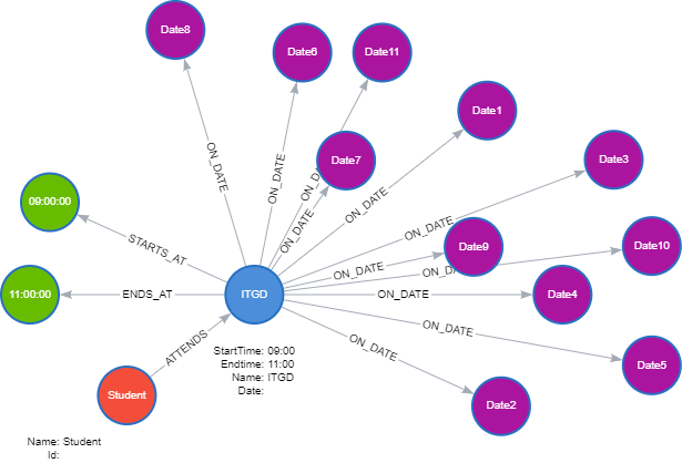
Graph Structure:
- 1 Activity node
- 11 Date nodes - shared by ALL activities on those dates.
- 2 Time nodes (09:00 and 11:00) - shared by ALL activities on those times!
- Additional Relationships
- Activity -[:SCHEDULED_ON]-> Date (11 relationships)
- Activity -[:STARTS_AT]-> Time (11 relationships to 09:00)
- Activity -[:ENDS_AT]-> Time (11 relationships to 11:00)
// cypher structure
(Activity {Name: "ITGD"})
    -[:SCHEDULED_ON]-> (Date {date: "2024-01-03"})
    -[:SCHEDULED_ON]-> (Date {date: "2024-01-10"})
    ...
    -[:STARTS_AT]-> (Time {time: "09:00"})
    -[:ENDS_AT]-> (Time {time: "11:00"})
Key point: Relationships encode which activity happens when.
Pros:
- Increased Flexibility: Facilitates queries across time ranges and aggregations across time slots.
- Reduced Redundancy: Avoids replicating time information for activities occurring on the same date and time.
- Lower Node Count: Potentially fewer nodes overall compared to Option 1 as
dateandtimenodes are shared with all activities in the database.
Cons:
- Increased Model Complexity: Requires managing relationships between Activity, Date, and Time nodes.
- Potential Performance Overhead: Querying might involve traversing multiple relationships, impacting efficiency.
Option 3: Date and Time Block Nodes
Option 3 creates a single activity but instead of individual start and end time nodes, we use predetermined timeBlocks encompassing both. For example, if using 30-minute blocks, we would have a node for “09:00-09:30” and another for “09:30-10:00”, etc.
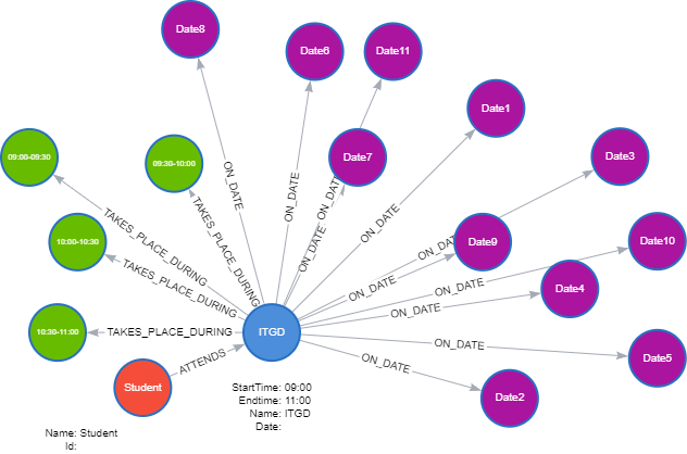
Graph Structure:
- 1 Activity node
- 11 Date nodes
- 4 Timeblock nodes (09:00-09:30, etc.) - shared by ALL activities on those times!
- Additional Relationships
Activity-[:SCHEDULED_ON]->Date(11 relationships)Activity-[:TAKES_PLACE_DURING]->timeBlock 09:00-09:30(11 relationships)Activity-[:TAKES_PLACE_DURING]->timeBlock 09:30-10:00(11 relationships)- …
// cypher structure
(Activity {Name: "ITGD"})
    -[:SCHEDULED_ON]-> (Date {date: "2024-01-03"})
    -[:SCHEDULED_ON]-> (Date {date: "2024-01-10"})
    ...
    -[:TAKES_PLACE_DURING]-> (TimeBlock {timeBlock: "09:00-09:30"})
    -[:TAKES_PLACE_DURING]-> (TimeBlock {timeBlock: "09:30-10:00"})
    -[:TAKES_PLACE_DURING]-> (Timeblock {timeBlock: "10:00-10:30"})
-[:TAKES_PLACE_DURING]-> (Timeblock {timeBlock: "10:30-11:00"})Pros:
- Granular Time Representation: Enables analysis at specific time intervals
- Easier Time Calculations: Duration is encoded and allows for easy calculations.
Cons:
- Potential for Data Sparsity: Some time blocks might be sparsely populated, leading to storage inefficiencies.
- Potential for High Node Codes: Lots of
TimeBlocksif using small intervals - Less flexible: Timeblocks are not dynamic.
Variations
StartTime and Duration: This option simplifies the model by representing time using only StartTime and DurationInMinutes properties on the Activity node, omitting explicit EndTime nodes. This approach is suitable for duration-based queries but it is limiting in that it is more difficult to query events occurring at specific times, overlapping time ranges or on end-times.
// cypher structure
(Timeblock {name: "09:00-11:00", start: 09:00, end: 11:00, duration:120})
(Timeblock {name: "10:30-11:30", start: 10:30, end: 11:30, duration:60})
(Timeblock {name: "11:00-12:00", start: 11:00, end: 12:00, duration:60})
Time Chains: This option retains date and time nodes, but instead of having relationships from activity, the nodes are chained: activity -> startTime -> endTime.
Time as Relationship Property: This option stores time information as properties on the relationship between Activity and Date nodes. This approach is more compact but can be less intuitive and may limit the ability to query based on time.
Dynamic TimeBlocks: This variation does not pre-create timeblocks based on a set interval (e.g. 30 minutes). They are created dynamically as required by the data and what already exists. For example, activities at 09:00-11:00, 10:30-11:30 and 11:00-12:00 would require these TimeBlocks:
Summary
| # | Option | Pros | Cons |
|---|---|---|---|
| 0 | Direct transfer (Normalised) | Simple | Minimal benefits (for time calculations) |
| 1 | Unique Occurrences | Simple, direct | High node count, complex time pattern queries |
| 2 | Date & Time Nodes | Lower activity node count, good for time-based queries | More complex relationships |
| 3 | Date & TimeBlock Nodes | Granular, easier duration calculations | Potentially high node count, sparsity if blocks are fine-grained |
Given the proof-of-concept scope of this project, I chose to proceed with Option 1. While this approach can lead to node proliferation, it offers the most straightforward implementation for exploring fundamental time-based queries and insights. It also acts as an easy jumping off point for exploring any of the other options.2
Footnotes
“Normalization is the process of organizing data in a database. It includes creating tables and establishing relationships between those tables according to rules designed both to protect the data and to make the database more flexible by eliminating redundancy and inconsistent dependency.” (helenclu, 2024)↩︎
Some of the above variations are explored in Appendix-Student Clashes↩︎