Graph vs Relational Data Models
As outlined in the project aims, my hypothesis is that graph-based approaches have the potential to offer new insights and efficiencies in timetable analysis. This section will briefly explore the theoretical underpinnings of graph data structures and their application to the domain of university timetabling.
Relational Models
Tables, Joins and the Limits of Interconnectedness
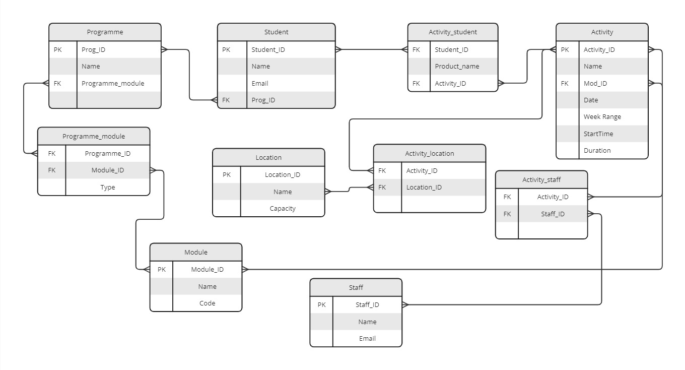
Relational databases, using SQL1 as their query language, have long been the go-to for managing data, including timetabling information. They structure data into tables, where rows represent instances of entities (e.g. individual rooms, staff, or students) and columns represent entity attributes (name, capacity, email, etc.).
Relationships between these entity tables are established through foreign keys, forming links between tables. This often involves intermediary “relationship” tables to handle the many-to-many nature of timetabling data (e.g., a student attends many activities, and an activity has many students) (Khan et al., 2023;Sokolova, Gómez and Borisoglebskaya, 2020).
While robust and well-understood, relational databases start to show their limitations when dealing with the highly interconnected nature of timetables:
Join Complexity: Even seemingly simple queries, like “find students attending a specific lecturer’s class in a particular building,” require joining multiple tables. As queries become more nuanced, the number of joins increases, often impacting performance, especially with large datasets.
Rigidity: Relational databases rely on a predefined schema, making them less adaptable to evolving needs. Adding new entities or relationships is not possible without disrupting existing queries and applications.
Graph Models
Embracing interconnectedness
In contrast to the rigid table structure of relational databases, graph databases offer a more intuitive and flexible approach for representing interconnected data like timetables. They utilise:
- Nodes: Represent entities. These are often the “nouns” like activity, room, staff, student.
- Edges: Represent relationships between nodes. These are often the “verbs” like TAUGHT_BY, ENROLLED_IN, SCHEDULED_AT, OWNED_BY.
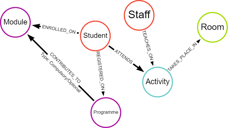
This node-and-edge structure inherently reflects how timetabling elements connect. Instead of relying on cumbersome joins, relationships are directly encoded in the data model itself. This results in several advantages:
- Natural Representation: Graph databases visually and conceptually mirror the relationships inherent in timetables, making them easier to understand and query.
- Relationship-Centric Queries: Graph databases are optimised for traversing and analysing relationships. Queries that would require multiple joins in a relational database often become significantly simpler and faster in a graph database.
- Flexibility: The schema-less or schema-optional nature of most graph databases allows for greater flexibility in data modeling. New entities or relationships can be added effortlessly without impacting existing structures or queries (Nan and Bai, 2019; Webber, Eifrem and Robinson, 2013).
Comparing queries
Example Insight: Find all students attending a specific lecturer’s class in a particular building
Representative queries have been written in SQL and Cypher to find this insight. The SQL query is much longer and requires six joins, each coming at a computational cost.
SQL Query
SELECT DISTINCT ss.[FirstName], ss.[LastName], ss.[Email]
FROM [RDB_MAIN2223].[rdowner].[V_STUDENTSET] ss
INNER JOIN [RDB_MAIN2223].[rdowner].[V_ACTIVITY_STUDENTSET] acts ON ss.[Id] = acts.[StudentSetId]
INNER JOIN [RDB_MAIN2223].[rdowner].[V_ACTIVITY] a ON acts.[ActivityId] = a.[Id]
INNER JOIN [RDB_MAIN2223].[rdowner].[V_ACTIVITY_LOCATION] al ON a.[Id] = al.[ActivityId]
INNER JOIN [RDB_MAIN2223].[rdowner].[V_LOCATION] l ON al.[LocationId] = l.[Id]
INNER JOIN [RDB_MAIN2223].[rdowner].[V_BUILDING] b ON l.[BuildingId] = b.[Id]
INNER JOIN [RDB_MAIN2223].[rdowner].[V_ACTIVITY_STAFF] ast ON a.[Id] = ast.[ActivityId]
WHERE ast.[StaffId] = 'StaffID'
  AND b.[Name] = 'BuildingName';
Cypher Query
In contrast, the Cypher query pattern is much simpler - written in one line (MATCH pattern). The query is more intuitive and easier to understand, especially for those unfamiliar with the database schema.
MATCH (s:Student)-[:ATTENDS]->(a:Activity)<-[:TEACHES_ON]-(st:Staff),
      (a:Activity)-[:TAKES_PLACE_IN]->(r:Room)
WHERE st.last_name = "LecturerLastName" AND r.building = "BuildingName"
RETURN s.first_name, s.last_name, s.email
Key Differences and Implications
| Feature | Relational Model | Graph Model |
|---|---|---|
| Data Structure | Tables with rows and columns | Nodes and edges |
| Schema | Rigid, predefined | Flexible, schema-less or schema-optional |
| Relationship Handling | Foreign keys, joins | Direct connections (edges) |
| Query Performance | Can be slow for relationship-heavy queries | Optimised for traversing relationships, potentially faster |
| Data Modeling | Less intuitive for interconnected data | Naturally represents complex relationships |
| Adaptability | Less adaptable to schema changes | More flexible, accommodates evolving data needs |
These advantages position graph databases as a powerful tool for uncovering insights hidden within complex, interconnected datasets like university timetables.
Footnotes
Structured Query Language (Wikipedia contributors, 2024)↩︎